Benchmarking local LLMs: what an RTX 2080Ti can actually do
Two quantized models, one eight-year-old GPU, and what the prefill/decode split reveals about attention vs. state-space costs.
Running large language models locally used to mean either a cloud API or a GPU with far more VRAM than most people own. This weekend I benchmarked two quantized models: one at 27 billion parameters, one at roughly 4 billion, on an RTX 2080 Ti, a card that's eight years old with 11GB of VRAM. Both ran. I wanted to actually measure how well, across two very different model sizes, instead of just taking "it works" as the whole story.
Here's what makes that possible, what I tested, and what the numbers actually say.
Quantization: how both models got this small
A model's weights are normally stored as 16-bit or 32-bit floating point numbers: that's what the model was trained in. Quantization takes those weights and represents them with far fewer bits, trading some precision for a much smaller file and less memory bandwidth needed to run it. A model quantized to 4-bit uses roughly a quarter of the storage of its 16-bit original; a model quantized all the way to 1-bit uses roughly a sixteenth.
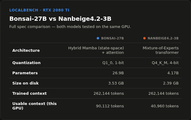
The two models I tested sit at opposite ends of that spectrum. Both fit comfortably inside 11GB of VRAM. Neither would fit anywhere close to that space running at full precision: a 27B model at 16-bit would need roughly 54GB just for the weights, before accounting for anything else the GPU needs to hold during inference.
What "running it locally" actually means
Running a model locally means the weights and the inference engine both live on your own hardware: nothing is sent to a third-party server to generate a response. I'm using llama.cpp, an open-source inference engine that's become the standard way to run quantized GGUF-format models on consumer GPUs (and CPUs, if you don't have a GPU at all). Some model architectures aren't supported in mainline llama.cpp yet, so both models here run on separate forks maintained for their specific architectures: that's a normal part of running less mainstream models locally right now.
The two models
Both models were trained on a 262,144 token context window, but neither can use all of it here: VRAM runs out before the model does. I found the real ceiling on this GPU with a binary search: load progressively larger contexts until it segfaults, then reduce it. Bonsai's ceiling is around 98K tokens, Nanbeige's around 45K. I run both with a safety margin below that, since failures past the ceiling are hard crashes, not an out-of-memory error.
How I benchmarked them
I used llama-bench (llama.cpp's built-in benchmarking tool) at three prompt depths: 512, 4,096, and 16,384 tokens, each followed by 128 generated tokens, 3 repetitions per depth. Every request to a model has two distinct phases: prefill, where the model processes the entire prompt before generating anything, and decode, where it generates the reply one token at a time. Time to first token (TTFT) is the wall-clock consequence of prefill: how long you actually wait before seeing a word.
Results
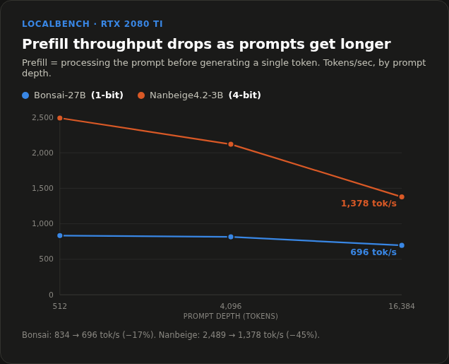
Prefill throughput falls as the prompt gets longer, for both models.
Decode barely reacts to any of this.
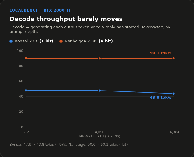
That decode number is worth pausing on for another reason: this GPU is eight years old, and 90 tok/s (or even Bonsai's 44 tok/s on a 27B model) is still a genuinely usable speed. The reason it holds up has to do with what decode actually taxes. Generating one token at a time means streaming the model's weights and the KV cache out of VRAM over and over: decode is bottlenecked by memory bandwidth, not raw compute. The RTX 2080 Ti has unusually high memory bandwidth for a consumer card, even by today's standards: a 352-bit memory bus rated at 616 GB/s, a spec several newer, cheaper cards have actually shipped with less of, since Nvidia has narrowed memory buses on more recent mid-range dies to cut cost. Prefill, which leans much more on raw compute across many tokens at once, is where a newer GPU's generational gains would actually show up; decode has less to gain from a compute-focused upgrade, because bandwidth was never this card's weak point to begin with.
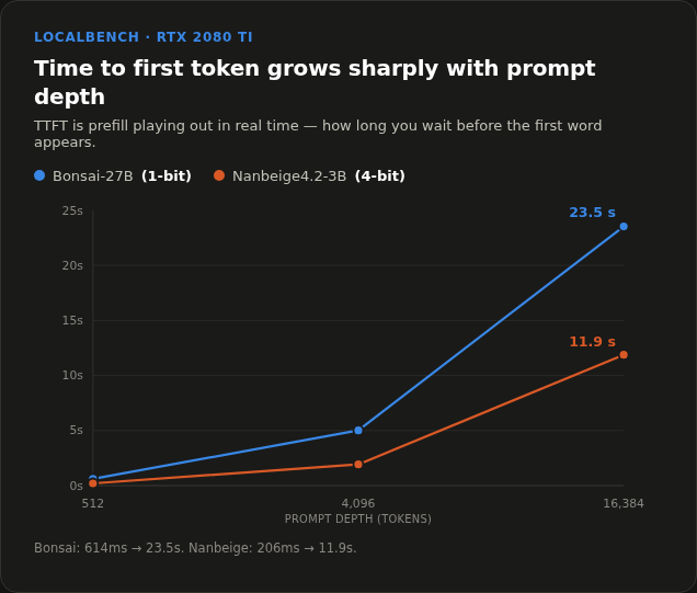
This is what a user actually feels. Time to first token is prefill's real-world cost, and since prefill is the phase that degrades, TTFT is where the pain shows up.
Why the gap: attention vs. state-space math
The 17% vs. 45% difference in how much prefill degraded is worth digging into, because it isn't just "the bigger model held up better." Bonsai is roughly six times larger than Nanbeige by parameter count: if size were the deciding factor, Bonsai should be the slower, more strained model at long context, not the one that degraded less.
The more likely explanation is architectural. Standard transformer attention has a cost that grows with the square of sequence length: to process token number 16,000, the model has to compute how it relates to all 15,999 tokens before it. Token 500 only has to look back at 499. That's why prefill throughput drops as prompts get longer even before you factor in there simply being more tokens to process: the per-token cost itself is rising.
Mamba, the architecture Bonsai partially uses, works differently. It's a state-space model (SSM): instead of attending back over every previous token, each new token updates a fixed-size internal state and moves on. The cost of processing token 16,000 is roughly the same as the cost of processing token 500, because the model isn't re-examining everything that came before; it's just carrying forward a compressed summary of it. That gives SSMs a cost that scales close to linearly with sequence length, instead of quadratically.
Bonsai isn't a pure state-space model; it's a hybrid, mixing Mamba layers with regular attention layers (a design pattern shared by models like Jamba and a handful of other recent hybrid architectures). The idea behind hybrids like this is to keep some attention layers around because pure SSMs can be weaker at precise long-range recall (needle-in-a-haystack lookups, for instance) while leaning on Mamba layers for the bulk of the sequence processing to keep the overall cost down. My guess is that's exactly what I'm seeing: only a fraction of Bonsai's layers pay something close to attention's quadratic-ish tax, while Nanbeige, a dense transformer, pays that tax on every layer, at every depth — and pays it twice over, since Nanbeige4.2-3B uses a looped-transformer design that passes hidden states through its physical layers a second time to approximate a deeper model, roughly doubling the attention work per token relative to a same-sized model run straight through once.
How much further a quantized KV cache pushes it
Everything above was measured with the default F16 KV cache: the per-token memory that stores each generated token's key/value vectors so later tokens can attend back to them without recomputing. That cache, not just the model weights, is what actually runs out of room first on this GPU. It can be quantized too, independently of the weights, via llama.cpp's -fa on -ctk <type> -ctv <type> flags: -fa (flash attention) is a hard prerequisite for the other two. I re-measured the real ceiling the same way as before (binary search to the point of a hard crash, not a guess) at Q8_0 and Q4_0, re-running F16 in the same session for a like-for-like baseline rather than reusing the numbers from the section above: the two F16 figures differ slightly (session-to-session variance, not a contradiction) precisely because they come from separate benchmark runs on different days.
| Model | KV cache | Context ceiling | Decode @ 16K tok/s | Δ vs F16 |
|---|---|---|---|---|
| Bonsai-27B | F16 | 98,304 | 42.2 | — |
| Bonsai-27B | Q8_0 | 155,648 (+58%) | 41.9 | -0.9% |
| Bonsai-27B | Q4_0 | 262,144 (full trained context, +167%) | 41.1 | -2.6% |
| Nanbeige4.2-3B | F16 | 45,056 | 84.3 | — |
| Nanbeige4.2-3B | Q8_0 | 77,824 (+73%) | 89.4 | +6.0% |
| Nanbeige4.2-3B | Q4_0 | 141,312 (+214%) | 89.0 | +5.5% |
The headline is that this was nearly free either way: decode speed held essentially flat for Bonsai and, if anything, ticked up for Nanbeige. I don't have a confident explanation for why quantizing the cache would make Nanbeige faster rather than just cheaper on memory. Either way, in exchange for at most a small decode cost, Bonsai went from 98K usable tokens to its entire 262K trained context at Q4_0, and Nanbeige more than tripled its ceiling.
Q8_0 is what I've since made the default for both models day-to-day: a good balance of headroom and safety margin.
Where this leaves things
Both of these are real, usable models, running with meaningful context windows, entirely on an 8-year-old consumer GPU. That's the actual headline here. The prefill/decode split is worth understanding if you're building something on top of this (long documents and RAG pipelines pay their cost up front, not throughout), but it's a detail underneath the bigger point: this class of model, at this level of capability, now fits on hardware most people already have.